Progress Update 2

Great job! You are now able to successfully identify which category an image most likely falls under.

To verify that your code is correct up to this checkpoint, please compare your code against the example code provided below.

Compare Your Code

Before moving on, please check your Google Colab notebook against the code below:

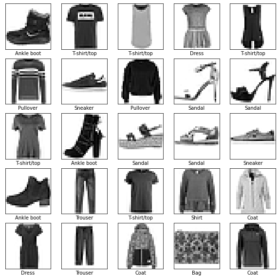
plt.figure(figsize=(10,10)) #sets the image size to 10x10 pixels
for i in range(25): #displays first 25 images with their class name
    plt.subplot(5,5,i+1)
    plt.xticks([])
    plt.yticks([])
    plt.grid(False)
    plt.imshow(train_images[i], cmap=plt.cm.binary) 
    plt.xlabel(class_names[train_labels[i]])
plt.show() #shows images with their labels

#Building the Neural Network
model = keras.Sequential([ 
    keras.layers.Flatten(input_shape=(28, 28)), 
    keras.layers.Dense(128, activation='relu'),
    keras.layers.Dense(10)
])

model.compile(optimizer='adam',
              loss=tf.keras.losses.SparseCategoricalCrossentropy(from_logits=True),
              metrics=['accuracy'])

model.fit(train_images, train_labels, epochs=10) 

Epoch 1/10
1875/1875 [==============================] - 4s 2ms/step - loss: 0.4990 - accuracy: 0.8247
Epoch 2/10
1875/1875 [==============================] - 4s 2ms/step - loss: 0.3754 - accuracy: 0.8658
Epoch 3/10
1875/1875 [==============================] - 4s 2ms/step - loss: 0.3374 - accuracy: 0.8771
Epoch 4/10
1875/1875 [==============================] - 4s 2ms/step - loss: 0.3110 - accuracy: 0.8859
Epoch 5/10
1875/1875 [==============================] - 4s 2ms/step - loss: 0.2935 - accuracy: 0.8903
Epoch 6/10
1875/1875 [==============================] - 4s 2ms/step - loss: 0.2823 - accuracy: 0.8942
Epoch 7/10
1875/1875 [==============================] - 4s 2ms/step - loss: 0.2682 - accuracy: 0.9002
Epoch 8/10
1875/1875 [==============================] - 4s 2ms/step - loss: 0.2575 - accuracy: 0.9041
Epoch 9/10
1875/1875 [==============================] - 4s 2ms/step - loss: 0.2479 - accuracy: 0.9074
Epoch 10/10
1875/1875 [==============================] - 4s 2ms/step - loss: 0.2417 - accuracy: 0.9088
<tensorflow.python.keras.callbacks.History at 0x7f2b4a7cb7b8>

test_loss, test_acc = model.evaluate(test_images,  test_labels, verbose=2)

print('\nTest accuracy:', test_acc)

313/313 - 0s - loss: 0.3358 - accuracy: 0.8825

Test accuracy: 0.8824999928474426

probability_model = tf.keras.Sequential([model, tf.keras.layers.Softmax()])

predictions = probability_model.predict(test_images)

predictions[7] #Returns the index with highest probability, depends on the index value.

array([3.5166186e-06, 5.8611111e-12, 7.3947496e-04, 3.9665038e-06,
       2.8206115e-03, 9.7542063e-08, 9.9643230e-01, 8.2940481e-11,
       1.2411938e-07, 2.7266096e-09], dtype=float32)

np.argmax(predictions[7]) # This returns the index value with the highest predictions

6

test_labels[7]  # This is the index value returned by the test dataset
                # (That we are comparing against)

6

class_names[6] # This is the category name of the image that has the highest probability

'Shirt'

Now that we are able to classify the category of an individual piece of clothing using your model, we will now visualize these predictions by creating a bar plot for a specified image.